IEEE TRANSACTIONS ON VISUALIZATION AND COMPUTER
GRAPHICS 1077-2626/98/$10.00 © 1998 IEEE
Vol. 4, No.
1: JANUARY-MARCH 1998, pp. 55-70
Modeling, Animating, and Rendering
Complex Scenes Using Volumetric Textures
*![[PDF ICON]](marcsvt_files/pdficon.gif)
Fabrice Neyret
Abstract![[mdash]](marcsvt_files/mdash.gif) Complex repetitive scenes containing forests,
foliage, grass, hair, or fur, are challenging for common modeling and
rendering tools. The amount of data, the tediousness of modeling and animation
tasks, and the cost of realistic rendering have caused such kind of scene to
see only limited use even in high-end productions. We describe here how the
use of volumetric textures is well suited to such scenes. These
primitives can greatly simplify modeling and animation tasks. More
importantly, they can be very efficiently rendered using ray tracing with few
aliasing artifacts. The main idea, initially introduced by Kajiya and Kay [9], is to represent a pattern of 3D
geometry in a reference volume, that is tiled over an underlying surface much
like a regular 2D texture. In our contribution, the mapping is independent of
the mesh subdivision, the pattern can contain any kind of shape, and it is
prefiltered at different scales as for MIP-mapping. Although the model
encoding is volumetric, the rendering method differs greatly from traditional
volume rendering: A volumetric texture only exists in the neighborhood of a
surface, and the repeated instances (called texels) of the reference
volume are spatially deformed. Furthermore, each voxel of the reference volume
contains a key feature which controls the reflectance function that
represents aggregate intravoxel geometry. This allows for ray-tracing of
highly complex scenes with very few aliasing artifacts, using a single ray per
pixel (for the part of the scene using the volumetric texture representation).
The major technical considerations of our method lie in the ray-path
determination and in the specification of the reflectance function.
Complex repetitive scenes containing forests,
foliage, grass, hair, or fur, are challenging for common modeling and
rendering tools. The amount of data, the tediousness of modeling and animation
tasks, and the cost of realistic rendering have caused such kind of scene to
see only limited use even in high-end productions. We describe here how the
use of volumetric textures is well suited to such scenes. These
primitives can greatly simplify modeling and animation tasks. More
importantly, they can be very efficiently rendered using ray tracing with few
aliasing artifacts. The main idea, initially introduced by Kajiya and Kay [9], is to represent a pattern of 3D
geometry in a reference volume, that is tiled over an underlying surface much
like a regular 2D texture. In our contribution, the mapping is independent of
the mesh subdivision, the pattern can contain any kind of shape, and it is
prefiltered at different scales as for MIP-mapping. Although the model
encoding is volumetric, the rendering method differs greatly from traditional
volume rendering: A volumetric texture only exists in the neighborhood of a
surface, and the repeated instances (called texels) of the reference
volume are spatially deformed. Furthermore, each voxel of the reference volume
contains a key feature which controls the reflectance function that
represents aggregate intravoxel geometry. This allows for ray-tracing of
highly complex scenes with very few aliasing artifacts, using a single ray per
pixel (for the part of the scene using the volumetric texture representation).
The major technical considerations of our method lie in the ray-path
determination and in the specification of the reflectance function.
Index TermsVolumetric textures, complex geometry,
levels of detail.
1. INTRODUCTION
The usual approach to geometric modeling consists of interactively
specifying component object meshes or surfaces, trajectories, deformations,
and materials. This approach is suitable for scenes of low to moderate
complexity, but it becomes problematic for complex, natural scenery due to the
enormous amount of data to specify. This work is also tedious for the modeler,
because the data may be repetitive and requires unnecessarily precise
knowledge, such as the position of each grass blade on a hill. Special-purpose
procedural tools exist to generate some families of shapes, but these are
often inflexible in the control the user has over a model.
More importantly, the usual rendering
methods tend to be very inefficient for highly complex scenes because
rendering cost is proportional, sometimes polynomially, to the number of
primitives. Furthermore, the small size of primitives, often occupying a small
fraction of a pixel, creates high-frequency signals that lead to very
noticeable aliasing artifacts and which are costly to avoid: There should be
at least as many rays launched per pixel as the number of primitives which
project onto a pixel. Some recent works propose solutions for walkthroughs at
interactive rates, using image caching dynamically [25] or precomputed [22]. These methods are not well
adapted to the high quality rendering of complex scenes poorly structured
(e.g., forest), where parallax effects and specular highlights are reluctant
to be cached.
Conversely, some dedicated procedural
rendering tools such as particle systems [21], [20] can be used to efficiently render
some complex shapes, at the expense of using a limited repertoire of shading
or reflectance models.
Volumetric textures can
provide a good trade-off between generality and efficiency: The key concept,
from the user's point of view, is the mapping of a replicated volumetric
pattern onto an underlying surface. Such a pattern encodes a sample of the
geometric material to be represented, such as a patch of grass, foliage, fur,
etc. This texturing process naturally distinguishes several scales of
specification: The local or fine scale is specified by the 3D pattern, the
medium scale is given by the mapping function, and the smooth or coarse scale
corresponds to the underlying surface shape (as shown in Fig. 1). The family of shapes handled
by this approach are objects that sit within a layer in the neighborhood of a
surface, like a thick skin, representing a kind of repetitive complexity. The
approach appears to be a good fit for a variety of natural objects, as
illustrated by our results.
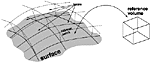
Fig. 1. The mapping of texels.
The seminal work on volumetric textures
by Kajiya and Kay [9] was matched in their implementation
to the modeling of fur. The texture mapping process was restrictive, in that
each texel fits exactly on a bilinear patch of the surface. More importantly,
the rendering computations were prohibitively expensive because of the volume
traversal at full resolution. We review this model in Section 2.
The motivations for our representation
are represented in Section 3. As described in Section 4, our representation
permits the encoding of any kind of shape in the volumetric pattern (as shown
in Fig. 2), and it provides a multiscale
representation akin to MIP-mapping which facilitates prefiltering at different
(see also [11]). As explained in Section 5, it
offers a much less restricted mapping from texture elements onto a surface in
a manner that is independent of the mesh subdivision, just as for regular 2D
textures (see also [13]). In this section, we also mention
some technical issues such as how to deal with color, and how to decrease
apparent periodicities in texture replication. We describe in Section 8 how to
convert shapes from their usual (geometric) representation to texels (see also
[13]), and, in Section 7, how to extend
the approach to the animation of complex scenes (see also [10]). The material in this paper
derives from the author's PhD thesis [14] (in French), and consolidates and
expands on the results presented in [10], [11], [13].
.gif)
Fig. 2. Sketch of our alternate geometry encoding: five
blades of grass, encoded at various resolutions (the rendering will choose the
one to be used according to the distance). The bottom figures show what is
stored: an opacity and a normals distribution function (NDF) in each voxel.
The integration of the Phong illumination model on the normals distribution
gives the reflectance, so that one can say that the distribution controls the
way the light is reflected. For clarity, the top figures retain illustrations
of the corresponding virtual geometry.
2. PREVIOUS WORK
Some of the basic principles of volumetric textures, for which our work can
be seen as an extension, have arisen in three lines of research:
- The texture mapping concept applied using an explicit 3D pattern was
introduced by Kajiya and Kay [9] in 1989, and extended by various
authors. The terminology volumetric texture and texel also
derives from this work. We present these early representations in Section
2.1.
- MIP-map texture multiscaling scheme has been introduced for 2D color
textures by [28]. We discuss the MIP-mapping
approach and its limitations in Section 2.2.
- Local reflectance modeling, especially in the scope of representing the
photometric behavior of subpixel geometric scales, has been previously
studied for haze [1] and surfaces [16], [6], as we will see in Section
2.3.
2.1 Early Volumetric Textures
Kajiya and Kay introduced volumetric textures in 1989 [9] in order to model fur. The key idea
was to represent the 3D material (fur) by a cubic reference volume, to be
mapped onto a surface (like a thick skin). The copies of the reference volume,
named texels, are fitted upon the bilinear patches of the surface,
and are deformed in order to stick to each other (see Fig. 1). A texel is, thus, a trilinear
deformation of the cubic reference volume. The volume itself is a 3D array of
voxels. Each voxel encodes the local geometry (a hair) by specifying an
opacity, a frame, and a canonical reflectance function (here, the one of a
cylinder). As there are nothing but parallel hairs in the volume, the frame
and the reflectance function are constant, so that only the opacity is really
stored in the volume. The combing of the fur is achieved using texels
deformation. The authors present a seminal image of a Teddy Bear, which
required a dozen CPU hours on an IBM3090 mainframe at that time.
Shinya proposed an anisotropic opacity
by storing in each voxel the opacity along the three canonical directions [24], to be maintained in a multiscale
way. However, the paper does not explain explicitly how to deal with the
reflectance information. Noma applies nondeformed texels to encode at various
scale procedurally generated trees consisting of sparse facets [15], using a multiscale scheme able to
switch from real geometry to texels as a function of the viewing distance.
2.2 Mip-Mapping and Its Limitation for Relief
Data
The MIP-mapping scheme has been introduced by Williams in 1983 [28] in the purpose of filtering 2D
image textures; however, it can be generalized to other surface attributes. It
consists of precomputing the surface attribute data (e.g., a color) at
multiple resolutions. The color to be seen in a screen pixel results from the
integration of whatever is visible in the cone starting from the eye and
passing through this pixel. This cone covers an area on the shape to be
rendered, so that the correct shading is obtained by integrating the local
illumination equation on this surface. The idea of prefiltering consists of
factoring the illumination equation (usually the Phong model): Assuming that
only the considered parameter varies within the pixel area and that this
parameter appears on a linear form in the equation, one can put the constant
term out of the integral so that one has only to integrate this parameter on
the given area. For the color, this means that integrating Phong with the
color varying along the surface area which corresponds to a screen pixel is
(almost) equivalent to using the average color in one single Phong evaluation.
Then, the integrals corresponding to different scales are precomputed, and
directly used at rendering time, thus providing a quasi correct imageand, consequently,
anti-aliasedwith a
single ray per pixel. For the MIP-mapping technique, the area of integration
is approximated by its bounding square, and the precomputed scales are the
power of two reductions of the texture resolution. When the optimal scale to
be used falls between two computed scales, one has to interpolate between the
two precomputed images of parameters (i.e., two smoothed color images in the
original paper).
Prefiltering in the fashion described
above presupposes that integrating the data to obtain a multiscale
representation is easily accomplished. That was the case for color or
transparency texture with which MIP-mapping is usually used, because one has
just to preintegrate the colors as explained above, as it is a linear
parameter of the Phong local illumination model. But, if one would want to use
a map containing geometrical data, such as normals or depth, this would no
longer works as these parameters are not linear in the equation (averaging
normals or depth would give a smoother relief, which is not the same as a
smoother image of the original relief. Typically, a rough surface is darker
than a smooth one).
As a remark, the MIP-mapping technique
is convenient and easy to program (it is even available on some graphics
hardware). It does not provide a perfect filtering, however, as it assumes a
square filtering kernel, whereas many situations mandate nonisotropic kernels.
For instance, on the border of a sphere, the texture is compressed a lot in
one direction and not in the other one. This implies that more pixels of
texture are covered in the compressed direction (the ones that vanish behind
the sphere), so the kernel should be larger in this direction, and also that
the weight of the compressed texture pixels should be smaller. More
complicated prefiltering methods like SAT [4] or NIL [5] exist to address some of the
deficiencies of the MIP-map filter. Buchanan [3] also specifically deals with the
filtering in the 3D case (i.e., volumes of texture). We do not discuss these
methods as they do not fit our needs, which are the ability to filter data
that is not simply a color and the necessity of minimal computation at
rendering time.
The multiscale reference volume
representation we use can be considered, in some respects, to be analogous to
3D MIP-mapping. However, we store a kind of geometrical information in the
voxels of our volumetric texture, rather than a color. Thus, we are out of the
trivial case, which implies that we will have to define how to filter this
voxel content.
2.3 Reflectance Representation
Kajiya suggests, in [8], adapting the model which
represents the details according to the distance, by using explicit geometry
for close points of view, a texture for intermediate points of view, and a
reflectance model for distant points of view. Thus, the reflectance can be
used to represent subpixel geometry: A very small object, such as a single ice
crystal in snow, can be observed through its reflective behavior, despite the
fact that it is too small for one to see its shape. As a remark, this implies
that polygonal decimation is not a good strategy in the scope of realistic
rendering: From a distant point of view, the shape of a corrugated iron sheet
looks like a flat sheet, while the illumination is still quite different from
that of a flat sheet because of the normals. The same occurs for a rough
surface whose geometry is close to the one of a smooth surface, while the
reflectance is not (the former being darker). Becker and Max have proposed in
[2] such a kind of transition between
geometry texture and reflectance for bumpy surfaces. However, this cannot
easily apply to free 3D details, which cannot be expressed as height-fields.
In this spirit of representing geometry
by reflectance, Blinn has computed the reflectance of a haze made of
microscopic spheres [1], Poulin has encoded anisotropic
surface with areas of microscopic parallel cylinders [16], and Fournier has represented the
BRDF,1 caused by
microgeometry, using a local set of "Phong peaks" which can be filtered
according to distance [6].
In the same spirit, we represent the
subpixel geometry by a feature controlling the reflectance, stored in each
voxel of the volume.2 To encode this
reflectance, a 4D BRDF table is too expensive in terms of memory, while
microprimitives such as spheres or cylinders are too specific. The trade-off
will be to choose a parameterized family of functions which are generic
enough, and require few parameters to specify.
3. MULTISCALE GENERIC VOLUMETRIC TEXTURES
In this section, we present the motivations for our representation, and we
present our main choices as prepared in the previous sections.
The limitations of the early volumetric
texture model [9] were:
- hardcoded and specific reflectance functions, e.g., for fur;
- full-resolution volume data, making rendering costly and prone to
aliasing;
- strong assumptions about the mesh subdivision;
- no or few descriptions of how to specify the reference volume content;
- no specification of texel animation;
- the representations deal with shapes, but not with colors.
In order to cope with all these issues
and, thus, to turn the early volumetric textures into an efficient and generic
model, we have applied an MIP-map-like multiscaling scheme to this 3D data,
and we have extended both the microscopic aspect (the reflectance function)
and the macroscopic aspect (the mapping).
The MIP-mapping scheme consists of
precomputing the data at multiple resolutions. For a volume, this leads to an
octree structure, as shown in Fig. 3. Tracing a ray through the
reference volume requires accessing the voxel information at the appropriate
level of detail. As for MIP-mapping, this is done by selecting the two levels
corresponding to voxel sizes which bound the ray thickness and, then,
interpolating the two results. Thus, the rendering can be compared to a
cone-tracing, as all the data within the ray cone is taken into account to
compute the color of a pixel. The filtering abilities of the method go from
the scale where one texture pixel projects on one screen pixel (if the
viewpoint is closer, the lack of resolution of the texture will be visible) up
to the scale where the whole texture pattern projects on a single screen pixel
(if the viewpoint is farther, aliasing will occur and several rays will have
to be launched per pixel in such a way that each pattern receives at least
one).
.gif)
Fig. 3. Reference volume octree encoding. The space is
subdivided only where the data lies, at a level depending on the data
variations. Coarser resolutions of the data are also stored in the octree. The
ray will consider the pyramid level for which voxels fit the pixel size once
projected on screen, or coarser voxels if the data is not available at that
resolution.
Each voxel stores opacity and a feature
controlling the reflectance function. For each level in the octree, the
information is obtained by filtering (in a way to be defined later) the
equivalent information from the level below. For compacity, we want to model
the reflectance by a parameterized family of functions. Such a family needs to
have a group structure: The filtering of eight functions at low-scale has to
be represented by one function of the same family at larger scale. This is not
directly possible for the function used in [9], namely, the function that
simulates the reflectance of a cylinder (because the sum of the reflectance of
two nonparallel cylinders cannot be expressed as the reflectance of a mean
cylinder). Thus, making the reflectance function more generic is also
necessary in order to apply the MIP-mapping scheme.
We describe in Section 4 how to choose,
render, and filter a good reflectance function family, which is the key point
of the method, as this allows to concentrate in a voxel the average
photometric behavior due to smaller scales, thus making possible the
multiscale scheme.
We present in Section 5 the way to map
texels on surfaces the same way as regular 2D textures, without constraining
the mesh (thus extending the Kajiya and Kay's [9] method, where the mesh is made of
bilinear patches). We also deal there with color encoding. Once the pattern
encoding and the mapping are in place, the kernel of the representation is
complete. This will be the right place to sum up our volumetric texture
specification.
We sketch in Section 6 the whole
volumetric textures rendering scheme.
To turn the representation into a
usable tool, we have to define ways to model the pattern content and to
animate the texels. The animation specification is dealt with in Section 7.
Thanks to the texturing philosophy, modeling and animation can be described at
three different scales: the geometric scale (related to the underlying
surface), the mapping scale (related to texels deformation), and the
microscopic scale (related to the voxel content), which is the spirit of the
hierarchy of details [8].
We show in Section 8 how to build a
volumetric texture pattern from various kinds of existing geometric
description. Once again, despite the use of an octree which evokes classical
volumetric representation, one has to keep in mind that the nature of the
voxel content makes the problems quite different.
4. THE REFLECTANCE MICRO-PRIMITIVE
4.1 Choosing a Primitive
The reflectance primitive to be represented in a voxel simulates the
photometric behavior of the subpixel3 geometry which
lies in this area of space, and the opacity coefficient represents the
probability for a ray to be stopped. We require a family of reflectance
functions generic enough to represent the geometry within a voxel, but having
few parameters, because they will need to be stored in each voxel.
Particularly, it is convenient to define a 2D normals distribution function
(NDF) rather than a 4D BRDF. Moreover, since normals have a geometric nature,
this form can also easily handle modifications of the shape to be represented,
such as deformations (one just has to multiply the normals by the transpose of
the deformation Jacobian). Using a parameterized family of distributions
allows us to compress the representation even more. We have chosen to encode
the normals distribution by an ellipsoid, i.e., we consider the normals of a
given ellipsoid [11], or, to state it another way, we
store the ellipsoid which NDF represents well as the wanted NDF, instead of
the wanted NDF itself. The BRDF can be reobtained by integrating the Phong
model on this normals distribution; it's what will be done at rendering time.
So, our "feature" is this ellipsoid, which purpose is to encode the
reflectance behavior of each voxel.
The subpixel (and subvoxel) geometry,
that is, the part of the scene clipped in the voxel, referred to here as the
"local shape," is either a small object (e.g., a section of grass) or a
surface element (e.g., a facet). An oriented ellipsoid centered on origin has
only six parameters, allowing us to efficiently encode various kind of local
shapes, including planes, cylinders, spheres, etc. We choose to store as
parameters the two smallest ellipsoid axis, the third one being defined as
orthogonal and having a unit length (the ellipsoid scale carries no
information for our purpose). A quadratic form corresponds to this ellipsoid,
which can be represented by a 3 × 3 matrix Q (M is on the
ellipsoid if MtQM = 1). The value of the
distribution  in direction N is given from
Q by: fQ(N) =
det(Q-1)/(Nt
Q-1N)2 (see the proof in Appendix A).
We will see that we can define the filtering of this primitive. It is
important to remind the reader that our ellipsoid is not a real object (it has
no size or exact location, for instance), but is only a representation for a
local distribution of normals.
in direction N is given from
Q by: fQ(N) =
det(Q-1)/(Nt
Q-1N)2 (see the proof in Appendix A).
We will see that we can define the filtering of this primitive. It is
important to remind the reader that our ellipsoid is not a real object (it has
no size or exact location, for instance), but is only a representation for a
local distribution of normals.
To be noted is that an ellipsoid is
symmetric, while the normal distribution of an object clipped in the voxel may
not be, especially for large objects for which the voxel mainly contains a
surface element. However, the innexisting represented normals are oriented
toward the inside of such object, so they will not be visible (except on the
horizon of the shape at very low resolution, as one can see in Fig. 4). The main limitation of the
ellipsoid is, of course, the few degrees of freedom it has, which limits its
acuity in fitting details in distributions: If the normal distribution has two
strong peaks (e.g., when summing two facets), the ellipsoid will simulate a
single smoothed one in the middle direction. Thus, details are blurred. This
is the price for a compact representation. We present in Fig. 18 in Appendix B the plots of the
NDF of various ellipsoids.
.gif)
Fig. 4. Rendering of a texel containing two spheres. (a)
Resolution 323. (b) Resolution 1283. Note how each voxel
reflects the light as if the real geometry were there, because of the
reflectance encoding.
4.2 Rendering the Primitive
At rendering time, when a ray will go through the voxels according to the
global rendering scheme described in Section 6, we will have to accumulate the
illumination and opacity of each visited voxel. We define here how to compute
this "atomic illumination" of an ellipsoid attached to a voxel. The
illumination is the ratio of energy received from a light source and scattered
toward the eye by an object. The ellipsoid we consider here encodes the normal
distribution .xbm) which induced illumination is
which induced illumination is.xbm)
where d is the eye direction, ![[psgr]](marcsvt_files/psgr.gif) ( ) is the local illumination model (we use
Phong), and (N.d) is the visibility.4 Because the
visibility of a normal is the same whether it is taken on the initial shape
clipped in the voxel or on the ellipsoid, this is equivalent to simply
integrating the illumination of the ellipsoid as if it was the shape to be
rendered:
( ) is the local illumination model (we use
Phong), and (N.d) is the visibility.4 Because the
visibility of a normal is the same whether it is taken on the initial shape
clipped in the voxel or on the ellipsoid, this is equivalent to simply
integrating the illumination of the ellipsoid as if it was the shape to be
rendered: .xbm) so that we never need to explicitly use the expression
fQ(N). Thus, we have the illumination of
a voxel, which simulates the subpixel geometry as shown in Fig. 4.
so that we never need to explicitly use the expression
fQ(N). Thus, we have the illumination of
a voxel, which simulates the subpixel geometry as shown in Fig. 4.
Because integrals on ellipsoids seldom
have a closed form, we use a uniformly-sampled numerical integration with 16
samples. The rectangle which bounds the apparent ellipse is easy to obtain:
Its dimensions correspond to the eigenvalues of the ellipse quadratic form
Q', which is obtained from the quadratic form Q of the
ellipsoid and the eye direction d by Q' = Q .xbm) QddtQ/dtQd.
Each sample on the ellipsoid is obtained by solving the second-degree
polynomial corresponding to the ray-ellipsoid intersection (see Fig. 5) as detailed in [11].
QddtQ/dtQd.
Each sample on the ellipsoid is obtained by solving the second-degree
polynomial corresponding to the ray-ellipsoid intersection (see Fig. 5) as detailed in [11].
.gif)
Fig. 5. Numerical integration of the ellipsoid
illumination.
We also use the ellipsoid to estimate
the variations of the opacity depending on the direction. This anisotropic
part is obtained by dividing the apparent surface of the ellipsoid relative to
its mean apparent surface. The real opacity is, then, the mean opacity (stored
in the voxel) times this ratio. The apparent surface is ![[pgr]](marcsvt_files/pgr.gif) times the surface of the bounding
rectangle computed above. The mean apparent surface is approximated by the
average from the three mains axes ri, i.e.,
times the surface of the bounding
rectangle computed above. The mean apparent surface is approximated by the
average from the three mains axes ri, i.e., .xbm)
The light arriving at the voxel where
the ellipsoid stands is obtained by launching a shadow ray that is treated the
same way as a regular ray (i.e., it is also a cone). We use a lower
resolution, i.e., a rougher level in the MIP-map, by multiplying the computed
ray aperture by a user-defined coefficient (usually two in our images). This
allows us to save computation time (shadow rays volume traversal can be very
important, especially when the sun is low on the horizon), and also to get
easily smoothed shadows, which is better for the image quality.
4.3 Filtering the Primitive
When several child voxels are merged to obtain the average information for
their parent in the octree, one has to integrate the voxels contents. This is
simple in the case of opacity (we accumulate the values that represent the
mean opacity


